Skip links

Trading Strategy for USD JPY using Historical Volatility and VWAP

Introduction

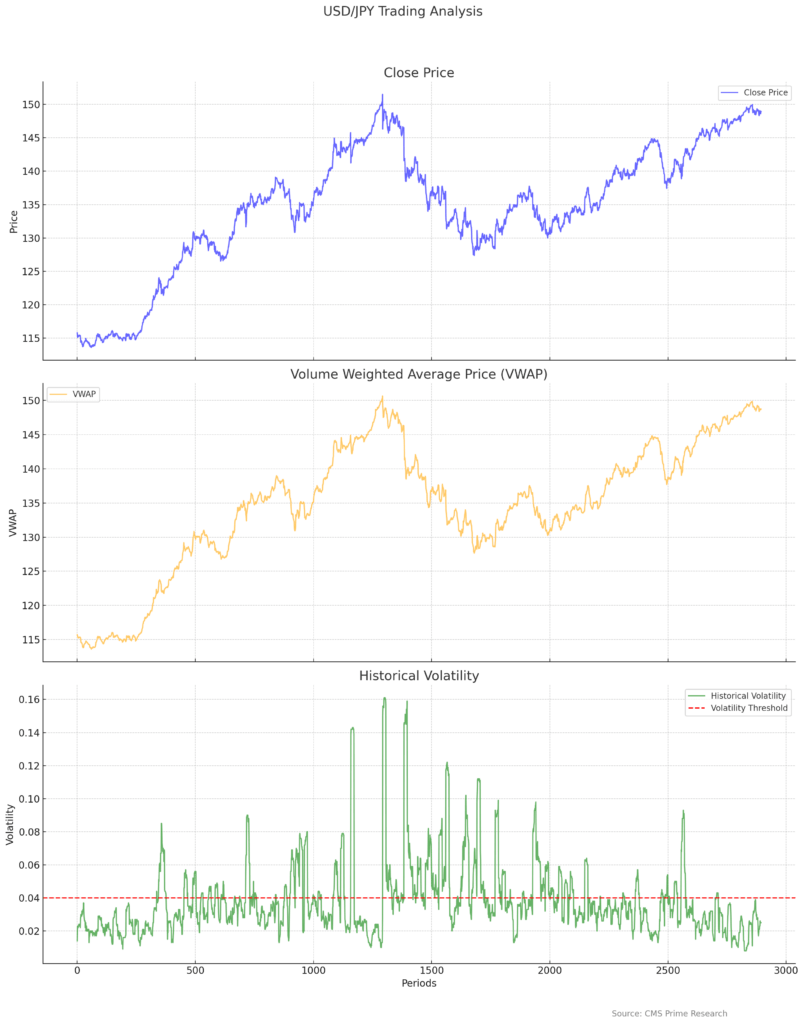
Understanding Historical Volatility and Volume Weighted Average Price (VWAP) is crucial for traders and investors as these metrics provide valuable insights into market trends and risk levels.

Historical Volatility (HV) is a statistical measure of the dispersion of returns for a given security or market index over a specific period of time. It is calculated by determining the average deviation from the average price of a financial instrument in the given time period. The higher the historical volatility value, the riskier the security. However, risk can work both ways—bullish and bearish. Historical volatility does not specifically measure the likelihood of loss, but it does measure how far a security’s price moves away from its mean value. This measure is frequently compared with implied volatility to determine if options prices are over- or undervalued. Historical volatility is also used in all types of risk valuations. Stocks with a high historical volatility usually require a higher risk tolerance. High volatility markets also require wider stop-loss levels and possibly higher margin requirements.

On the other hand, Volume Weighted Average Price (VWAP) is a tool that traders use to track the average price of a security over a certain period of time. VWAP gives traders insight into how a stock trades for that day and determines, for some, a good price at which to buy or sell. It can also help traders and analysts gain insight into where the momentum is at a specific time frame. For example, if a stock reverses and has a clean breakout above the VWAP, the trader should look to cover the short because they may be on the wrong side of the trade; the momentum has shifted to the buy side because the sellers have let up.

In conclusion, understanding Historical Volatility and VWAP is essential for traders and investors as it helps them make informed decisions about their investments. These metrics provide insights into market trends, risk levels, and potential investment opportunities.

The Data:

The dataset contains 2895 entries and the following columns:

  1. Periods: An identifier for the time period.
  2. Tick Range: Numerical range of the tick (presumably the difference between high and low prices in a given period).
  3. Open: Opening price for the period.
  4. High: Highest price during the period.
  5. Low: Lowest price during the period.
  6. Close: Closing price for the period.
  7. VWAP: Volume Weighted Average Price.
  8. %K: A parameter, which might be related to a stochastic oscillator (common in technical analysis).
  9. %D: Another parameter often associated with the stochastic oscillator.
  10. Historical Volatility: A calculated measure of the price volatility.

Analysis to Consider before Backtesting

The correlation coefficients between the “Close” prices and the two variables are as follows:

1. Close Price and VWAP: (0.999)
2. Close Price and Historical Volatility: (0.071)

– Close Price vs. VWAP:
– The extremely high positive correlation ((0.999)) indicates that the “Close” prices and “VWAP” are almost perfectly linearly related. This is also visually evident from the graph we plotted earlier. The “Close” price and “VWAP” tend to move together, and a change in one is associated with a nearly identical change in the other.

– Close Price vs. Historical Volatility:
– The correlation coefficient is (0.071), which indicates a very weak positive linear relationship between “Close” prices and “Historical Volatility”. In practical terms, changes in historical volatility are not strongly associated with changes in the close price in a linear fashion.

These correlations suggest that while VWAP might be a very relevant factor to consider in strategies involving close prices, the historical volatility might not provide strong predictive power in a linear model for predicting close prices.

Backtesting and Results

First lets consider the 2 Conditions:

  1. Buy Condition:

    • VWAP > Close Price
    • Historical Volatility (HV) > 0.040
  2. Sell Condition:

    • VWAP < Close Price
    • Historical Volatility (HV) > 0.040
  • Initial Capital: $10,000
  • Total Hypothetical Profit/Loss: $14,063.54
  • Return on Capital: 140.64%
Trade Breakdown:
  • Total Trades: 164
  • Positive Trades: 111
  • Negative Trades: 53
Expected:
  • Positive Outlook: The strategy seems to have performed well hypothetically on this historical data, providing a substantial return on capital.
  • Risk: Despite the high return, risks such as consecutive losses (drawdown) and overfitting to historical data need to be considered.
  • Further Validation: It would be beneficial to validate the strategy using out-of-sample data to ensure that it is not overfitting the historical data.
  • Risk Management: Applying robust risk management is crucial, especially considering the leverage and rapid price movements in forex trading.
Backtest Results

In the realm of financial trading, developing and scrutinizing a strategy through various metrics and graphical representations is paramount to comprehend its potential efficacy and risks. Three vital graphical tools often utilized by traders and investors to evaluate the performance of a trading strategy over a specific historical period include the Equity Curve, Profit/Loss Distribution, and Cumulative Profits and Losses chart. Let’s delve into a succinct overview of each.

1. Equity Curve
  • The green line represents the growth of the initial capital over the number of trades.
  • The red dashed line indicates the initial capital.
  • The equity curve shows a generally upward trajectory, indicating that the strategy was hypothetically profitable over this historical data.
2. Profit/Loss Distribution
  • This histogram displays the distribution of profits and losses per trade.
  • The red dashed line represents the breakeven point.
  • The distribution shows a range of outcomes, both positive and negative, with a higher frequency of profitable trades.
3. Cumulative Profits and Losses
  • The green line represents the cumulative profits over the trades.
  • The red line represents the cumulative losses over the trades.
  • This plot illustrates how profits and losses accumulate over time, providing insight into periods of gains and drawdowns.
Deepdiving in the Metrics

The Important metrics we considered:

  1. Maximum Drawdown: The largest peak-to-trough drop in the equity curve.
  2. Sharpe Ratio: A measure that indicates the average return minus the risk-free return divided by the standard deviation of return on an investment.
  3. Sortino Ratio: Similar to the Sharpe Ratio but only considers the standard deviation of negative portfolio returns. It’s a risk-adjusted measure of a risk-free investment.
  4. Win Rate: The percentage of trades that were profitable.
  5. Average Win/Loss: The average size of profitable trades vs. losing trades.
  6. Profit Factor: The ratio of gross profit to gross loss.
Examination of the Results:
  • Maximum Drawdown: The largest decline from a peak to a trough in the equity curve, indicating a $768.25 loss.

  • Sharpe Ratio: A higher value (1.78) indicates a better risk-adjusted return.

  • Sortino Ratio: A higher value (2.38) shows a better return for the same unit of downside risk.

  • Win Rate: Approximately 68% of trades were profitable.

  • Average Win/Loss: On average, winning trades gained $349.83, while losing trades lost $467.31.

  • Profit Factor: The profits are 1.57 times the size of the losses.

Points to Consider:
  • Risk Management: Even with profitable metrics, it’s crucial to manage risk appropriately to safeguard against significant drawdowns.
  • Strategy Assessment: While these metrics provide a comprehensive view of the strategy’s performance on historical data, it’s vital to validate the strategy on out-of-sample data to ensure robustness.
Conclusion

The analytical journey through the intricacies of Historical Volatility and Volume Weighted Average Price (VWAP) unveils a compelling, yet cautionary tale of trading strategy development, spotlighting the imperative of intertwining metric-driven decision-making with rigorous validation and risk management. While the examined dataset and ensuing backtesting proffer an ostensibly prosperous strategy, yielding a hypothetical return on capital of 140.64%, it’s paramount to recognize the limitations and potential pitfalls enveloped in historical data and theoretical outcomes. The highly linear relationship between VWAP and closing prices alongside the weak correlation between Historical Volatility and closing prices brought forth a strategy that, though seemingly prosperous in a controlled, historical context, necessitates further scrutiny, especially through the lens of out-of-sample data testing and potential overfitting mitigation.

Amidst the optimism birthed by favorable metrics such as a Sharpe Ratio of 1.78, a Sortino Ratio of 2.38, and a win rate of 68%, resides an unyielding imperative for astute, continual strategy assessment and unwavering adherence to prudent risk management. Even with a strategy that demonstrates promise within a historical context, its practical, future application warrants a steadfast commitment to safeguarding against excessive financial exposure and ensuring that the strategy is resilient and adaptable to the ever-fluctuating landscapes of the financial markets. Thus, traders and investors are beckoned to traverse the exciting yet precarious pathways of strategy development with a mindset firmly planted in rigorous validation, continual refinement, and, fundamentally, an unassailable dedication to risk management.

Disclaimer: This is not an Investment Advice. Investing and trading in currencies involve inherent risks. It’s essential to conduct thorough research and consider your risk tolerance before engaging in any financial activities.